This tutorial demonstrate how captcp outperform wireshark for TCP flow analysis. This tutorial focus on throughput analysis for a specific TCP flow. In a separate tutorial I will demonstrate how Gnuplot can be tweaked to generate a nice image ready for web publishing or for your bachelor/master/phd thesis. The need for this tutorial arise from discussions with captcp users where I think that the workflow with captcp and Gnuplot is not ideal. So take this tutorial as a best practices tutorial. Sure, there will be other ways too.
So first we start to capture a TCP flow. As I mentioned in the captcp documentation it is always a good idea to capture network data and do a offline analysis of the data! And please don't forget to disable the offload capabilities of your network adapter! Read the section "What you see is NOT what you get" on the captcp homepage: research.protocollabs.com/captcp
tcpdump -i eth0 -w trace.pcap
pid=$!
wget http://www.example.com/large-file
kill $pid
This capture all data on device eth5 (please use your device) and save the packet trace in trace.pcap. Later we download a large file (say 10 Mbyte) and after all you just stop the capturing process. trace.pcap should now contain at least one complete TCP transfer including three-way-handshake, file transfer and termination. If any other network processes are running, like browser or cloud music players you will download that streams too.
Wireshark Throughput Analysis
We start with wireshark analysis. We open wireshark directly with the trace file. My packet capture file contains many different connection - 47 to be exact. Wireshark can show information about every TCP connection via Statistics &aarr; Conversation List / TCP (IPv4 & IPv6). The following screenshow show this:
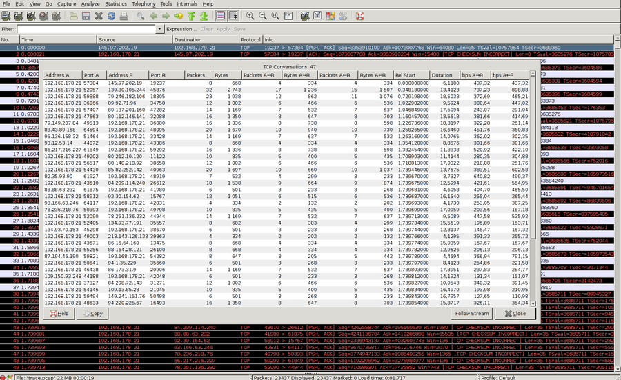
The problem is that we want to limit the throughput graph to exactly on connection. The standard Statistics / IO Graph is not usable because it will always show the IO impact for the whole capture. But with a trick we can bypass this by save the particular TCP stream to another dumpfile. Via right click on one packet in the TCP stream, followed by Conversation Filter / TCP we can limit the wireshark view to only this TCP stream. Something like the following filter should be displayed in the filter box:
(ip.addr eq 87.248.217.254 and ip.addr eq 192.168.178.21) and (tcp.port eq 80 and tcp.port eq 55173)
Next step is to save only the displayed packets. File / Specified Packets and Save. You will see the dialog inform you that there are captured and displayed packets. The number of displayed packets should match the expectations. Save this file as stream.pcap and open this file now. You should only see the particular packets - if not something went wrong and you should check the filter.
Now you can open Statistics / IO Graph and the image and the control elements should look like the following:
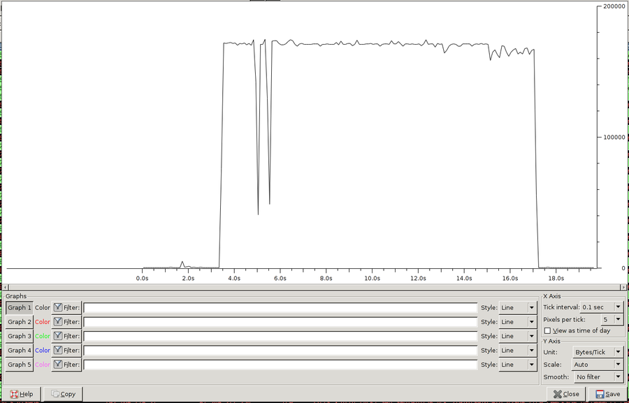
I set the tick interval to 0.1 seconds and increase the pixel per tick to 5 to display more details. Furthermore I change the Units from Packet/s to Byte/s.
You can save this image as PNG and voila. You can integrate the file in your thesis and thats all. You cannot modify the image afterwards (except Gimp). There is also no possibility to add a axis label or store the image in a vector format (PDF or SVG).
In the next section I show how captcp can display the throughput of a particular TCP connection.
Captcp Throughput Analysis
To identify the TCP stream we start the statistic module of captcp:
captcp statistic trace.pcap
This list all TCP streams in the file. We search the list for the specific connection and remember the particular stream:
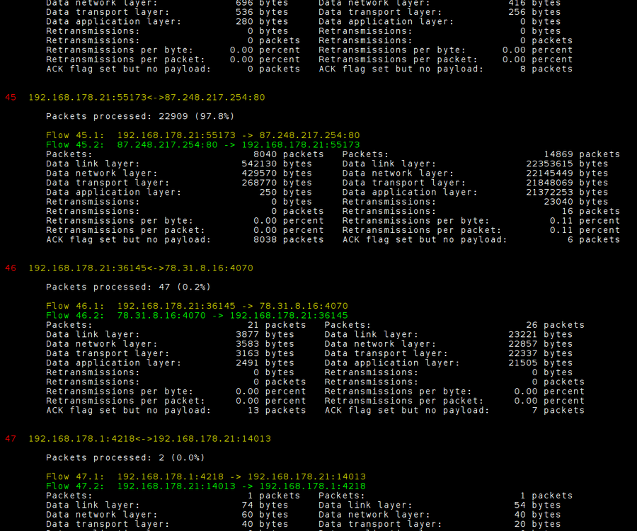
For trace.pcap flow 45.2 is the right one! Now we can start the throughput module and graph the data. First we generate the raw data and in a second step we start Gnuplot (via make) to generate the PDF file. To keep the workspace tidy we create a temporary directory to output all intermediate files. We name this directory simple "out".
mkdir out
captcp throughput -s 0.1 -i -f 45.2 -o out trace.pcap
cd out
make png
# view throughput.png
The generated PNG image look like the following:
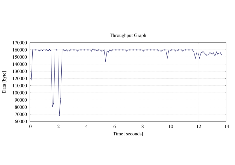
Arguments to captcp are s to specify the sampling interval - here 0.1 seconds. i mean initial and generate a Gnuplot environment to generate the image out from the raw data file (throughput.data). You MUST skip this flag if you modify the Gnuplot file (throughput.gpi). If not than the gnuplot file is overwritten each time you execute it. The f flag specify the flow and o the output directory where all file are generated.
I hope this help to print some nice throughput graphs! In a later tutorial I will show how you can modify the gnuplot file and start with some Gnuplot magic! ;-)
Questions? Ideas? Bugs? Email me