Description
Visualize the throughput of tracefile - or a selected connection - over time.
Options
| Short Option | Long Option | Description |
|---|---|---|
| -s <sample-length> | --sample-length <sample-length> | length in seconds (float) where data is accumulated (default: 1.0 second) |
| -m <mode> | --mode <mode> | layer where the data len measurement is taken. Valid options: goodput (application layer, default), transport-layer, network-layer or link-layer (Ethernet) |
| -u <unit> | --unit <unit> | units: bit, kilobit, megabit, gigabit, byte, kilobyte, megabyte, gigabyte, kibibit, mebibit, gibibit, kibibyte, mebibyte, gibibyte |
| -f <connections> | --data-flow <connections> | specify the number of relevant id's |
| -i | --init | create (overwrite existing) Gnuplot template and Makefile in output-dir |
| -o <output-dir> | --output-dir <output-dir> | specify the output directory |
| -h | --help | print this help screen and usage info |
Usage
In this example we use a trace file where 20MB data are uploaded. We start by a simple print to stdout. We use the default mode where the data is collected at application level. No Ethernet Header, IPv{4,6} Header nor TCP header is accounted. Just application level data (i.e. including HTTP overhead if HTTP protocol). We can change this default via --mode: application-layer, transport-layer or network-layer or valid options.
captcp.py throughput --stdio traces20.pcap
 1.0      1440.0
 2.0    149760.0
 3.0    125280.0
 4.0    129600.0
 5.0    123840.0
 6.0    139680.0
 7.0    149760.0
 8.0    156960.0
 9.0    151200.0
10.0    100800.0
11.0     74880.0
12.0    188640.0
13.0    133920.0
14.0     99360.0
15.0    112320.0
16.0    122400.0
17.0     97760.0
# total data (goodput): 2057600 byte (16.46 Mbit)
# throughput (goodput): 115693.10 byte/s (925.54 kbit/s)
What we see here is that the throughput is in average 925.54 kbit/s. Between start and second 1 we transfer 1440byte, between second 1 and 2 we transfer 149760.0 byte and so on. The throughput is relative stable over time,except between second 10 and 11 and a next time between 13 and 14. The last segment (second 16-17) can be ignored because connection shutdown is in progress.
But let us take a more exact look at the data. This time we increase the granularity by 2. We thus increase the sampling rate to 0.5 seconds. Additionally we choose to account IP and TCP overhead too.
captcp throughput --mode network-layer --sample-length 0.5 --stdio trace20.pcap
 0.5      1664.0
 1.0      1492.0
 1.5     89536.0
 2.0     66844.0
 2.5     66792.0
[...]
17.0     35248.0
17.5      1092.0
# total data (network-layer): 2191356 byte (17.53 Mbit)
# throughput (network-layer): 123213.82 byte/s (985.71 kbit/s)
Nothing special: the data is as expected. The sample length can be useful to spot gaps where the transmission stalls. This can happened on a larger scale when e.g. crosstraffic (another upload) is active. On the other side, the sample length option can be useful to check if there are some stop-and-wait behavior within the transmission. E.g. the sender is receiver limited and artificial throttle the connection within a second. Therefore is is often wise to increase the sampling rate (decrease sample delta time).
Now we skip the stdout generator and generate a image - an illustration is always good! Because it is the first time we pass the --init option. This will generate boilerplate Gnuplot files and a Makefile. Additionally we need a directory where all files are generated. We can use the actual directory by passing . to --output-dir but we want to keep the directories clean we create an additional directory, called throughput-analysis.
mkdir throughput-analysis
captcp throughput --init --output-dir throughput-analysis trace20.pcap
After the data is generated we can change the directory and simple type make. This generate a PDF file. Fine for zoom into details as well as an import graphic for LaTeX. Type make png generate a PNG file for further processing, e.g. website. The following illustration is the direct result:
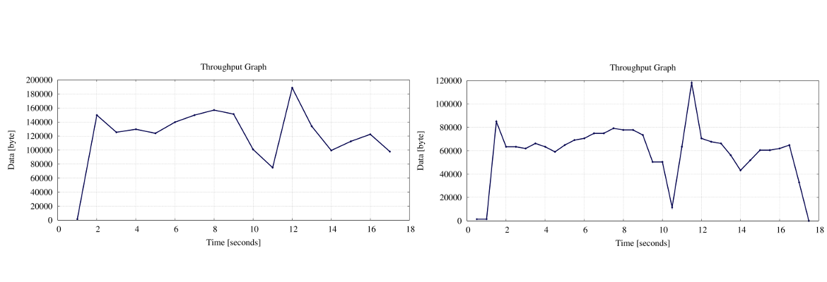
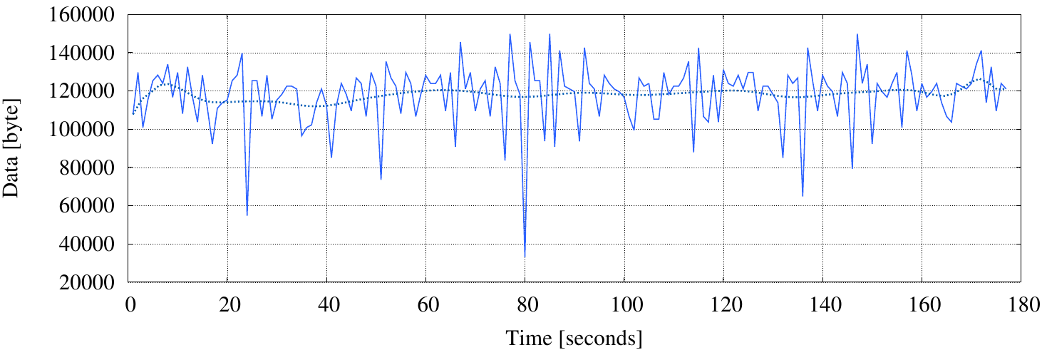
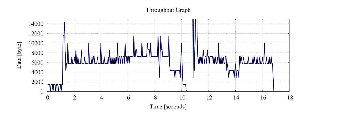
The last image set the sample-length to 0.05 and in the Gnuplot file (throughput.gpi), the yrange is limited (set yrange [0:15000]). Thats the throughput module! We will analyze this PCAP trace later with some other modules too.
Units
Captcp understand a vast number of units. Including all SI/IEC prefix. See Binary Prefix for a complete list. Note that lowercase/uppercase is important. Default is byte (thus byte per second). Binary prefixes are not widely used in network communication, but you are free to use it. Sometimes you see KiB/MiB (mainly counter related statistics). Here some examples:
captcp throughput -u byte     --stdio trace.pcap
captcp throughput -u kilobyte --stdio trace.pcap
captcp throughput -u Mbit     --stdio trace.pcap
captcp throughput -u mebibyte --stdio trace.pcap